Square Lattice Ising Model

The Ising Model is one of the earliest treatments of ferromagnetism in statistical mechanics. Although the model was first proposed by Wilhelm Lenz in 1920, it takes its name from one of Lenz's students, Ernest Ising, who made headway formalizing the 1-dimensional model.

Basic Definitions

Although many variations of this model exist, I will consider the model characterized by a square lattice of spins which can either be in the state \(1\) (spin-up) or \(-1\) (spin-down). Each spin is coupled to its nearest neighbors (above, below, left, right) with a constant, \(J_{i,j}\). In general cases, the coupling depends on the specific pair of spins, however this value will be the same for all pairs of spins in the model. The table below demonstrates one of the ways a \(3\times3\) lattice may be populated by the two spin states.

↓	↑	↓
↓	↓	↑
↓	↑	↓

Classically, the magnetization, \(M\), of a solid is defined as the volume density of magnetic dipole moments. Here, we will define the absolute magnetization, \(M\), of an \(N \times N\) configuration to be the absolute value of the average spin, \( \sigma_i \), per site. \[ M = \left| \frac{1}{N^2} \sum_{i = 0}^{N^2} \sigma_i \right| \] Additionally, the expression for the energy of our configuration in an external longitudinal field, \(h\) is: \[ E = -J \sum_{i,j} \sigma_i \sigma_j - h \sum_{i} \sigma_i \] From the equation above, we can predict at least three interesting cases:

1. J = 0. The energy is minimized by spins aligning with an external field. The coupling (or lack of coupling) between neighboring spins does not contribute to the energy. We expect to observe paramagnetic ordering of the system.
2. J < 0. Again, the energy is minimized by spins aligning with an external field. However, the coupling between neighboring spins does contribute to the energy, and is minimized by neighboring spins opposing each other. We expect the system to display antiferromagnetic ordering.
3. J > 0.(The case we will consider.) Once more, the energy is minimized by spins aligning with an external field. However, the coupling between neighboring spins does contribute to the energy, and is minimized by neighboring spins aligning with each other. We expect to observe ferromagnetic ordering of the system.

However, we will be considering the simplified case where there is no external field: \[ E = -J \sum_{i, j} \sigma_i \sigma_j \]

The Canonical Ensemble

Through the theromdynamic identity, we can show that for a particular system with a constant number of particles, \(N\), and constant volume \(V\), the temperature, \(T\), entropy, \(S\), and internal energy \(U\) are related by: \[ \frac{1}{T} = \left( \frac{\partial S}{\partial U}\right)_{N, V} \] Additionally, the entropy, \(S\), for a macrostate, \( \mu \), is defined in terms of the number of microstates associated with it: the multiplicity, \(\Omega\). \[ S(\mu) = k_B \ln(\Omega(\mu)) \] In order to study the behavior of the system across different temperature scales, we will consider our spin lattice to be in thermal equilibrium with a large heat reservoir at a temperature \(T\). The combination of the heat bath and spin lattice form a canonical ensemble when allowed to exchange energy with each other.

System \(\epsilon_S = U_0 - \epsilon_R\)

Heat Bath \(\epsilon_R = U_0 - \epsilon_S\)

On the figure above, the internal energy of both the reservoir and system are defined in complementary terms as the internal energy of the system is \(U_0 = \epsilon_R + \epsilon_S\).

In order to arrive at the probability of the system having an internal energy \(\epsilon_i\), we can consider the probability of the reservoir being in the energy state \(\epsilon_R = U_0 - \epsilon_i\). This value will be proportional to the number of states satisfying this condition, which is given by the multiplicity. \[ P_S(\epsilon_i) = P_R(U_0 - \epsilon_i) \propto \Omega(U_0 - \epsilon_i)\] Where the multiplicity can be expressed in terms of the entropy: \[ \Omega_R(U_0 - \epsilon_i) = \exp{ \left( \frac{S_R(U_0 - \epsilon_i)}{k_B} \right)} \] We can Taylor expand the entropy about \(U_0\) to first order taking \(\epsilon_i \ll U_0\): \[ S_R(U_0 - \epsilon_i) \approx S_R(U_0) - \epsilon_i \frac{d S_R}{d U} \] As \(N\) and \(V\) are constant we can refer to the thermodynamic identity to replace the derivative in the expression with inverse temperature: \[ S_R(U_0 - \epsilon_i) \approx S_R(U_0) - \epsilon_i \frac{1}{T} \] Returning the following for our probability: \[P_S(\epsilon_i) \propto \exp{\left(\frac{S_R(U_0) - \epsilon_i/T}{k_B}\right)} = \exp{\left(S_R(U_0) / k_B \right)} \exp{\left(- \frac{\epsilon_i} { k_B T }\right)} \] Which is a constant multiplied by a function of \(\epsilon_i\). We can show that for a set of \(\epsilon_i \) where the probability obeys \(P(\epsilon_i) \propto c~ f(\epsilon_i) \): \[ P(\epsilon_i) = \frac{f(\epsilon_i)}{\sum_i f(\epsilon_i)} \] Here our function of \(\epsilon_i\) is the Boltzmann factor:

And we introduce the partition function:

As the Ising Model can be described through a canonical ensemble, the probability of certain configurations of spins are determined by their respective energies for any temperature. The Hamiltonian of the system (in the absence of an external field) exhibits Z2 symmetry as the energy of the system is solely determined by the alignment of neighboring spins. If each spin is flipped (multiplied by -1), the sign of the total of all spins changes (and the absolute value of the total is the same), while the energy of the configuration remains the same. \[ E' = -J \sum_{i, j} (-\sigma_i) (-\sigma_j) = -J \sum_{i, j} \sigma_i \sigma_j = E \]

Markov Chain Monte Carlo Methods

One of the more interesting phenomena associated with ferromagnetism is the presence of a Curie temperature. Bringing a ferromagnet above this temperature induces a phase transition which can be observed as changes in the magnetic susceptibility and the loss of any spontaneous magnetization. This is part of the motivation for using statistical tools to study the influence of temperature on the system.

Depending on the temperature, thermal fluctuations will disorient spins away from their neighbors into alternate configurations with probabilities given by the Boltzmann factors. As the Boltzmann factor corresponding to a configuration with energy \(\epsilon_i\) is given by \(e^{-\frac{\epsilon_i}{k_B T}}\), each macrostate with energy \(\epsilon_i\) has a nonzero probability for \(T > 0\). This demonstrates the ergodicity of the system. As a direct consequence, we can calculate ensemble averages of the magnetization and energy on a sufficiently long trajectory of the system through phase space. As each of the transitions between states depends only on the current state of the system, it can be modelled by a Markov Process.

Additionally, seeking to sample from the equilibrium distribution, we seek an algorithm with the property of detailed balance. At equilibrium, the probability of transferring \(A \xrightarrow{} B\) will be equal to the probability of transferring \(B \xrightarrow{} A\). If our Markov Process has a stationary distribution, \(\pi\), then the following expression summarizes detailed balance:

Where \(\pi_i\) is the probability of being in state \(i\) given the stationary distribution \(\pi\) and \(p_{i \xrightarrow{} j}\) is the probability of transferring from state \(i\) to state \(j\) in one step given all possible transitions leaving state \(i\).

Metropolis-Hastings Algorithm

One such algorithm which satisfies the criteria above is the Metropolis-Hastings Algorithm. The system is sampled by considering the energy difference between the current state and a state in which a random spin is flipped.

1. Choose a random spin to flip.
2. Compute the change in energy, \(\Delta E\).
3. If \(\Delta E \lt 0\) accept new configuration.
4. Otherwise, pick a random \(r \) , \(0 \leq r \lt 1\).
   Accept proposed spin flip only if \(\exp(- \Delta E / k_B T) \gt r\).

Ultimately, the acceptance condition states that we flip the spin with a probability: \[ A(\Delta E) = \min \left(1, \exp{\left( \frac{-\Delta E}{k_B T} \right)} \right)\] To verify the condition of detailed balance for this algorithm, consider a proposed spin flip from a state with energy \(x\) to one with energy \(y\) where \( x \lt y\). Letting \(\beta = 1 / (k_B T) \), the probability of the configuration being in a state with energy \(x\) at temperature \(T~\) is: \[ P(x) = \frac{e^{- \beta x}}{Z} \] Where Z is the canonical partition function. Having \(\Delta E_{x \xrightarrow{} y} > 0\), The acceptance condition becomes: \[ A(\Delta E_{x \xrightarrow{} y}) = \min \left(1, \exp{\left( -\beta \Delta E_{x \xrightarrow{} y} \right)} \right) = \exp{\left( -\beta \Delta E_{x \xrightarrow{} y} \right)}\] The flow of probability from state \(x\) to \(y\) is the product of the acceptance condition and \(P(x)\): \[ \pi_x p_{x \xrightarrow{} y} = P(x) A(\Delta E_{x \xrightarrow{} y}) = \frac{e^{- \beta x}}{Z} \exp{\left( -\beta \Delta E_{x \xrightarrow{} y} \right)} = \frac{\exp(- \beta y)}{Z} \] For the reverse process, \(\Delta E_{y \xrightarrow{} x} = -\Delta E_{x \xrightarrow{} y}\) so that \(\Delta E_{y \xrightarrow{} x} \lt 0\). Therefore, this process is always accepted. We then find that: \[ \pi_y p_{y \xrightarrow{} x} = P(y) A(\Delta E_{y \xrightarrow{} x}) = \frac{\exp(-\beta y)}{Z} \left(1 \right) = \frac{\exp(-\beta y)}{Z} = \pi_x p_{x \xrightarrow{} y} \] And we have shown that the Metropolis-Hastings Algorithm satisfies detailed balance.

Verifying the Algorithm

In order to verify that the algorithm accurately samples from the partition function, we can compare the simulated expectation values \(\langle M \rangle\) and \(\langle E \rangle\) to the values computed analytically.

Recall that the energy of the system, as well as the magnitude of the magnetization, is invariant under the flipping of every spin. Working on a lattice with an odd number of spins, we can show that every configuration with a magnetization \(m_k > 0\) and energy \(E_k\) can be paired with a flipped configuration having magnetization \(-m_k\) and energy \(E_k\).

In order to compute the ensemble averages, we need a method to iterate over each configuration in the state space once and only once. First, we can notice, that for a grid containing \(N\) spins on each side, there is a total of \(N^2\) spins which can each be assigned one of \(2\) spins, bringing the total number of configurations to: \[\prod_{k=1}^{N^2} 2 = 2 ^ {\left(N^2\right)}\] Additionally, as each lattice site can be occupied by one of two spins, it is quite natural to represent each state as a binary number with \(N^2\) bits. In this representation the spins \(\{-1, 1\}\) are mapped to the bits \(\{0, 1\}\). Due to the symmetry of the system under spin inversion, we can cut the number of states to study in half by focusing on the first \(2 ^ {\left(N^2 - 1\right)}\) states. The other half of the states consists of states which are the one's complements of the first half of the states. As a result, the proportion of states having an energy \(\epsilon_i\) and absolute magnetization \(M_i\) in the first \(2 ^ {\left(N^2 - 1\right)}\) states is the same as the respective proportions in the last \(2 ^ {\left(N^2 - 1\right)}\) as well as in the entire state space.

The exact spectrum of energies for the 3x3 Ising model with fixed boundaries was computed by iterating over the first 256 states. I assigned each state a base-10 "identity" by mapping the sequence of spins (with indices increasing left to right then top to bottom) to a binary number with the most-significant bit corresponding to the spin in the state's zero index. The partition function was then computed for \(0 \leq \beta \leq 9.99\), which allowing a straightforward calculation of the relative probabilities for each microstate, as well as the expectation values of \(E\) and \(M\) as a function of \(\beta\).

These values were compared to the corresponding simulated values using the Metropolis-Hastings Algorithm. As each run is initialized with a random state (which we have no reason to believe is representative of the equilibrium state), the system is cycled through 1000 sweeps (each sweep being \(N^2 = 9\) update steps) before collection over 1000 sweeps. The following plots show the expectation values of energy and magnetization as a function of \(\beta\) for both the simulation and theory:

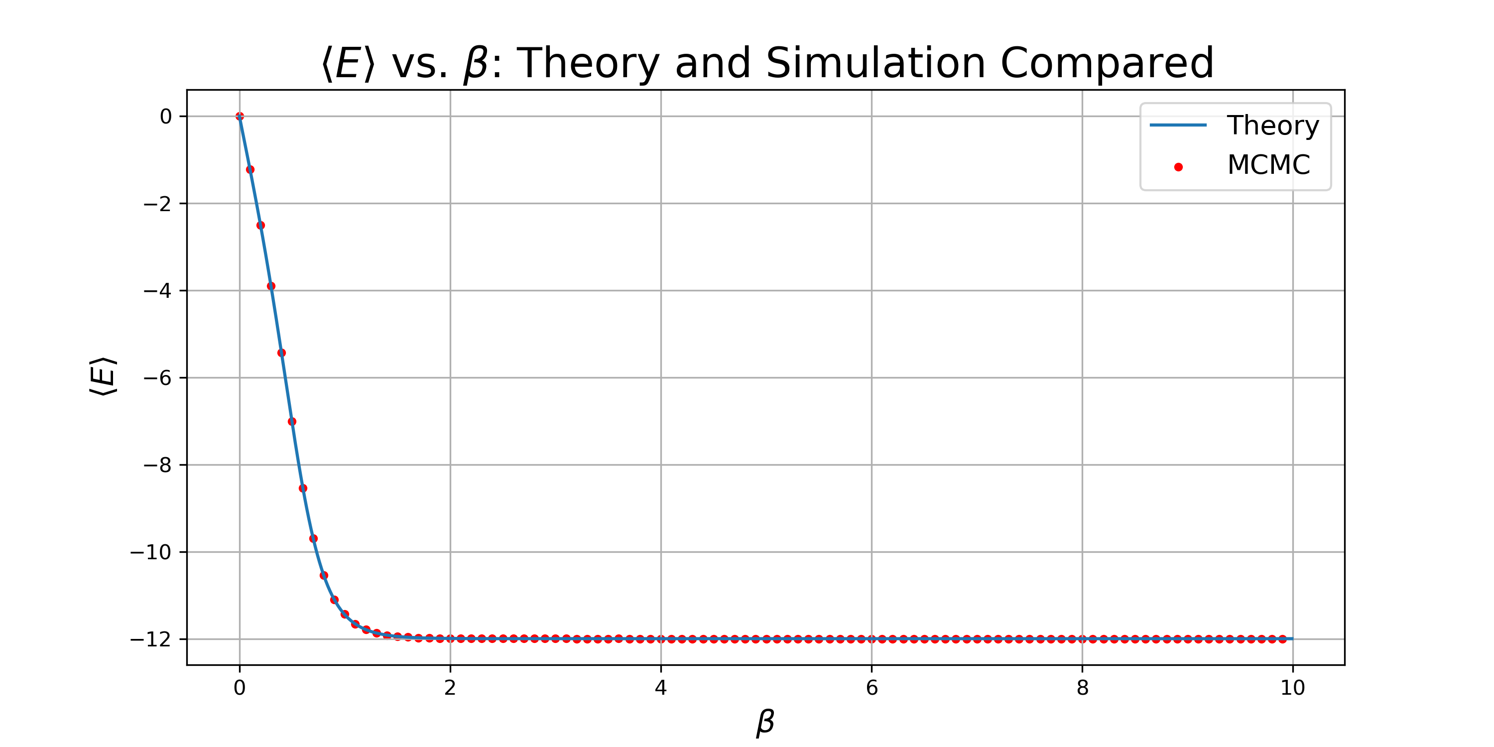
Both of the plots demonstrate a strong agreement between the simulation and theory across a range of temperatures. In order to confirm that my implementation of the Metropolis-Hastings algorithm approaches the desired equilibrium distribution, we can compare the relative occurences of each state in the simulation to the theoretical values. As the whole state space of microstates are available in the simulation, we need to map any state with an identity, \(i \gt 255\), to its ones' complement, \(i^* \lt 256\), in order to match the theoretical distribution over the reduced state space. The following plots compare the theoretical and simulated values across a comprehensive range of \(\beta\) values:

On each of the plots, the simulated probabilities of each microstate tend to cluster near the corresponding theoretical probabilities. However, the plots illustrate a trend of the simulation fitting the theory more accurately with increasing \(\beta\), which is confirmed by an analysis of the Kullback–Leibler divergence as a function of \(\beta\). The KL divergence allows us to quantify how "far" the simulated probability distribution, \(q\), is from the theoretical distribution \(p\). In the case of a discrete distribution, the expression for KL divergence is: \[D_{KL} = \sum_k p_k \ln \left( \frac{p_k}{q_k} \right)\]

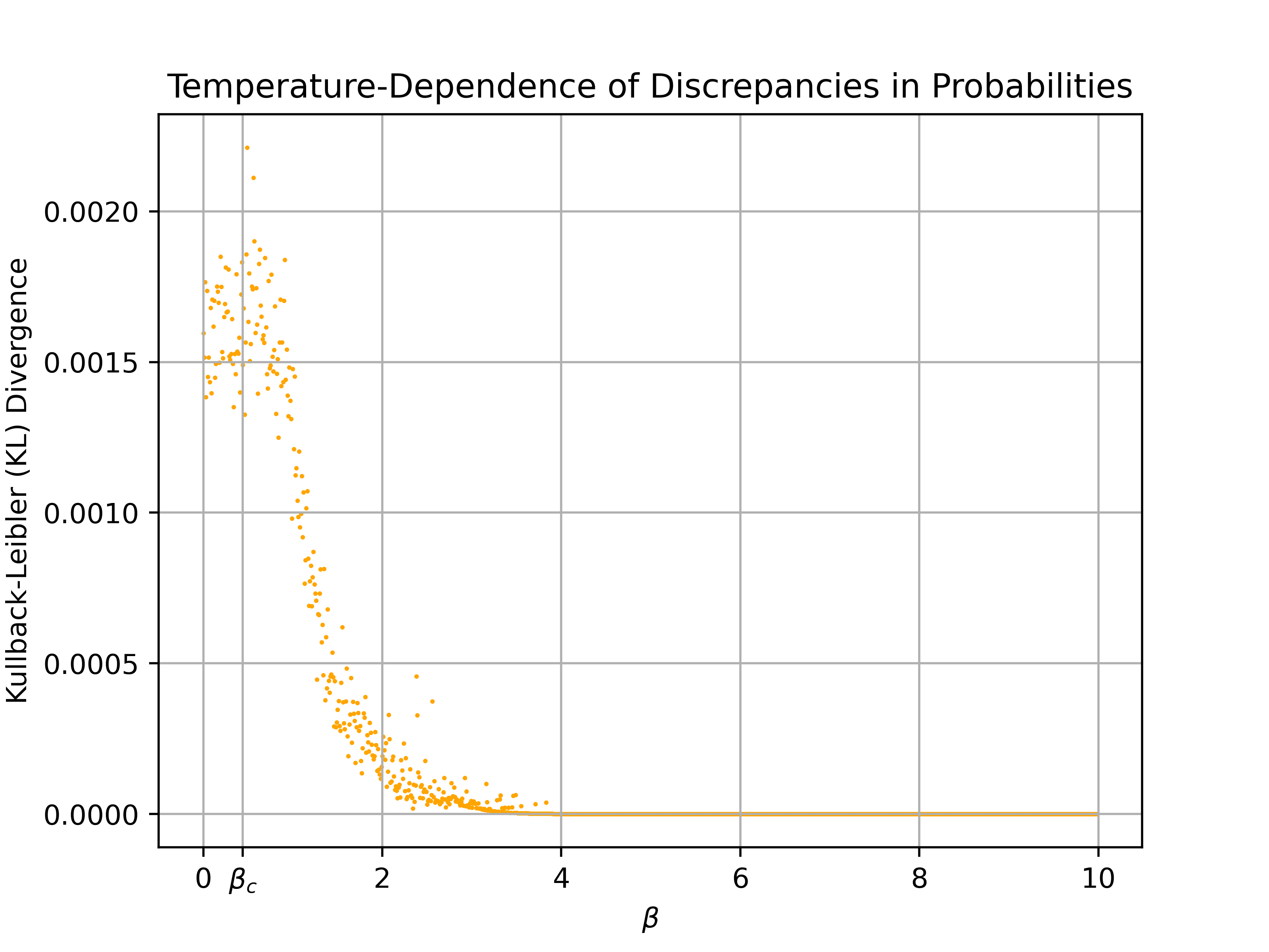
Note that the simulated distribution more closely approaches the theoretical distribution for higher values of \(\beta\), as demonstrated by the drop in KL divergence. Additionally, note how the distributions diverge around the critical value of \(\beta\), demonstrating the difficulty in using the Metropolis-Hastings algorithm around the phase transition. Around the critical point, the correlation length of the system diverges, making it difficult to capture the behavior of the system using local updates. However, the next section discusses the use of cluster aglorithms to combat the "critical slowing down" and other inefficiencies stemming from slow updates.

Improving Efficiency with the Wolff Algorithm

While the detailed proof is beyond the scope of this page, it is worth mentioning that certain algorithms, such as the Wolff Algorithm, can generate a Markov Chain that converges to a stationary distribution consistent with the Boltzmann distribution of the system. This is achieved by updating clusters of spins collectively rather than individual spins. The algorithm can be described as:

1. Choose a random spin to seed the cluster.
2. Draw a bond to one of the seed's nearest neighbors which share the same spin state.
   Accept the bond with a probability \(P = 1 - \exp(-2 \beta J)\).
3. Repeat step 2 once for each site added to the cluster until no more sites are added.
4. Flip the spins of each site in the cluster.

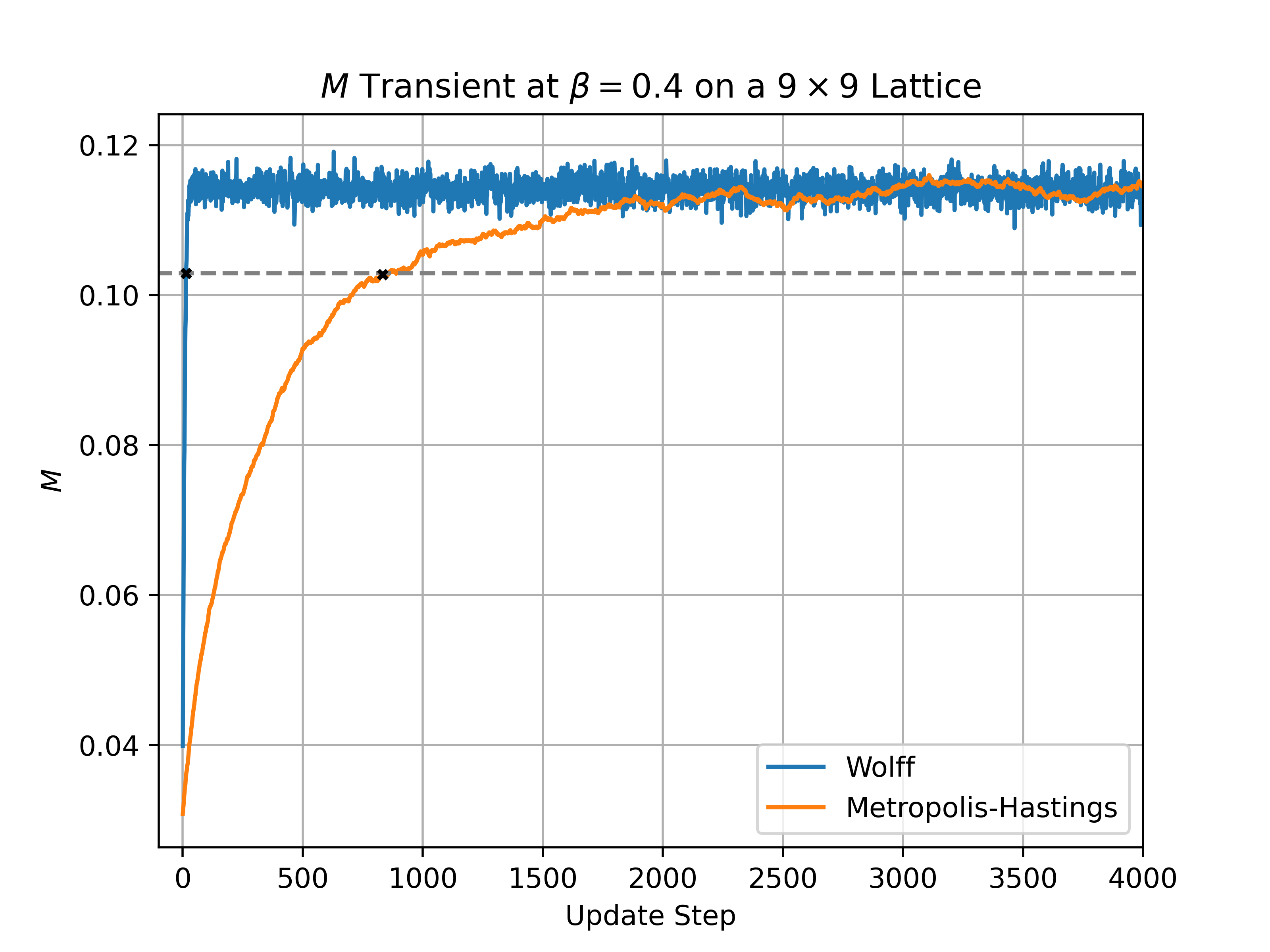
In addition to improved sampling around the critical point, the Wolff algorithm allows for a reduction in the number of time steps needed to reach a trajectory representative of the Boltzmann distribution. The figure below compares the evolution of \(M\) from an identical random initial state using the Wolff and Metropolis-Hastings algorithms. Note that the Wolff algorithm reached 90% of \(\langle M_{\beta=0.4} \rangle\) at 14 updates, while the MH algorithm took 833 updates.

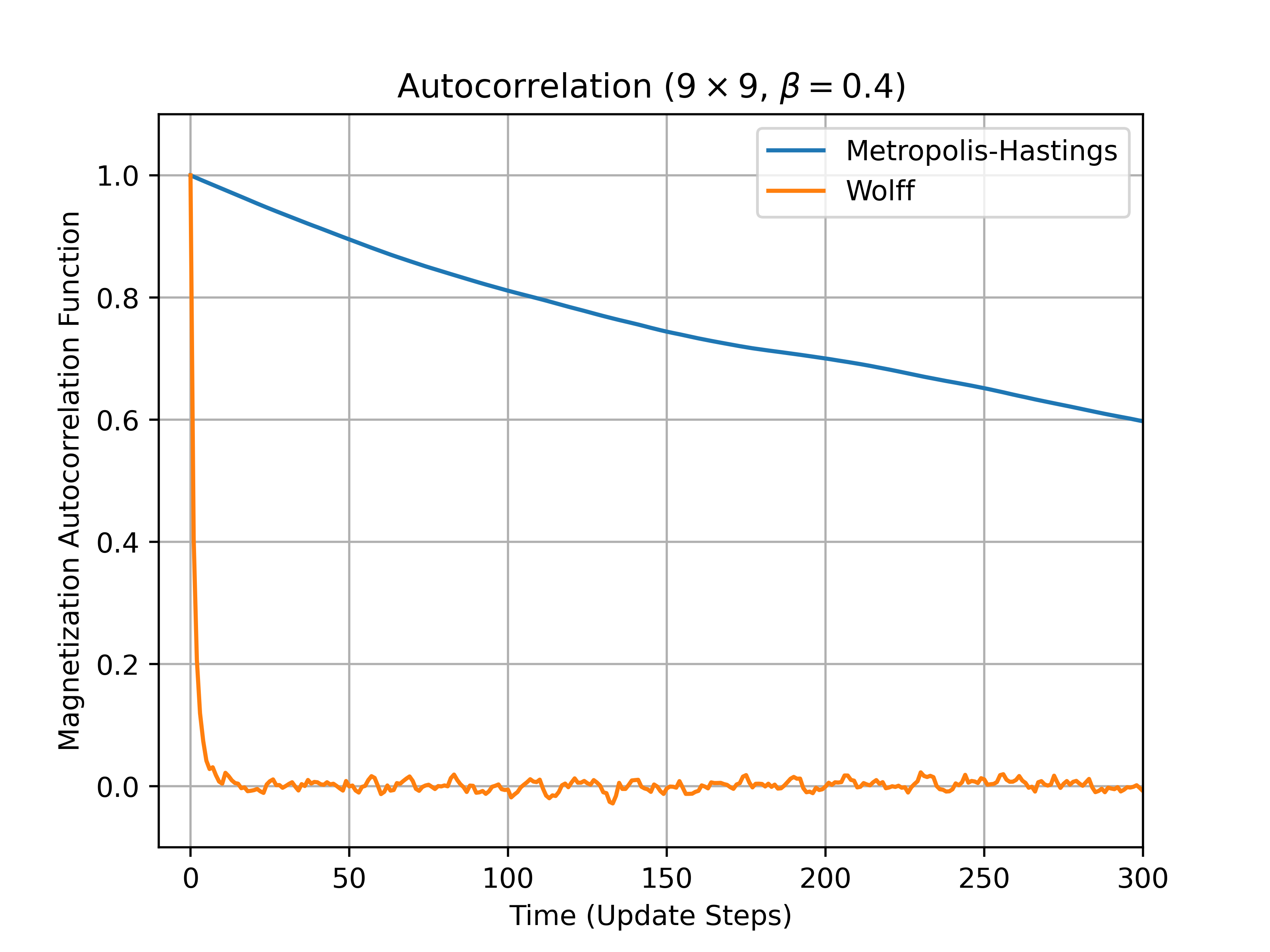
Additionally, note the reduction in autocorrelation times for the Wolff Algorithm:

Thanks to these improvements in efficiency, I will be using the Wolff algorithm for much of the remaining the investigations.

Sample Configurations

The following snapshots for different values of \(\beta\) illustrate the effect of temperature on the system. Each \(81 \times 81\) lattice was configured with the same initial state followed by 20 Wolff updates and 100 sweeps of Metropolis updates. For this simulation time scale, we can see the increasing disorder with temperature as the uniformly magnetized state disappears with decreasing \(\beta\). Then larger domains appear and are replaced with smaller domains until the state looks random.

Demonstrating a Phase Transition

In order to model the behavior of the system over a large range of temperatures, I used the Wolff algorithm to simulate a 41 x 41 grid over the range \(0 \leq \beta \leq 1\). The plot below illustrates the resulting energy and magnetization curves with the error bars denoting the standard deviation.

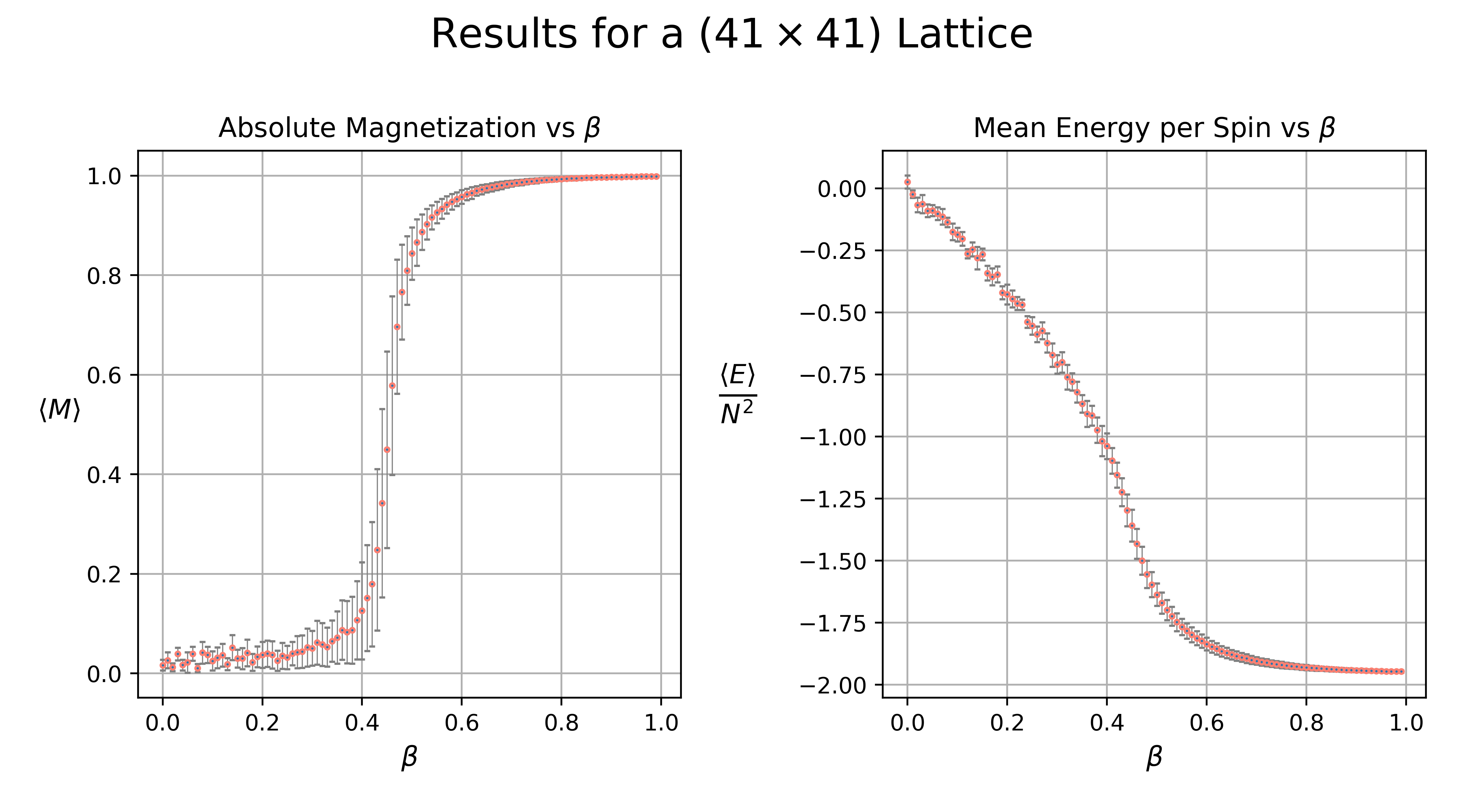
Note that as \(\beta \xrightarrow{} \infty\) (\(T \xrightarrow{} 0\)), the absolute magnetization tends towards 1, indicating a large-scale ordering of the spins. In the opposite limit, the disappearance of any large-scale ordering is suggested as \(\langle M \rangle \sim 0\).

In order to demonstrate the presence of a phase transition, we can look for a divergence in the specific heat, \(C_v\). For second-order phase transitions, the correlation length of the system greatly increases around the critical temperature. As a result, the influence of thermal fluctuations becomes larger. By working with the definition of the specific heat, \[C_V = \frac{d \langle E \rangle}{d T}\] we can arrive at the following result from the fluctuation-dissipation theorem (which is simpler to use for numerical simulations): \[C_V = \frac{\langle E^2 \rangle - \langle E \rangle ^2}{k_B T^2}\]

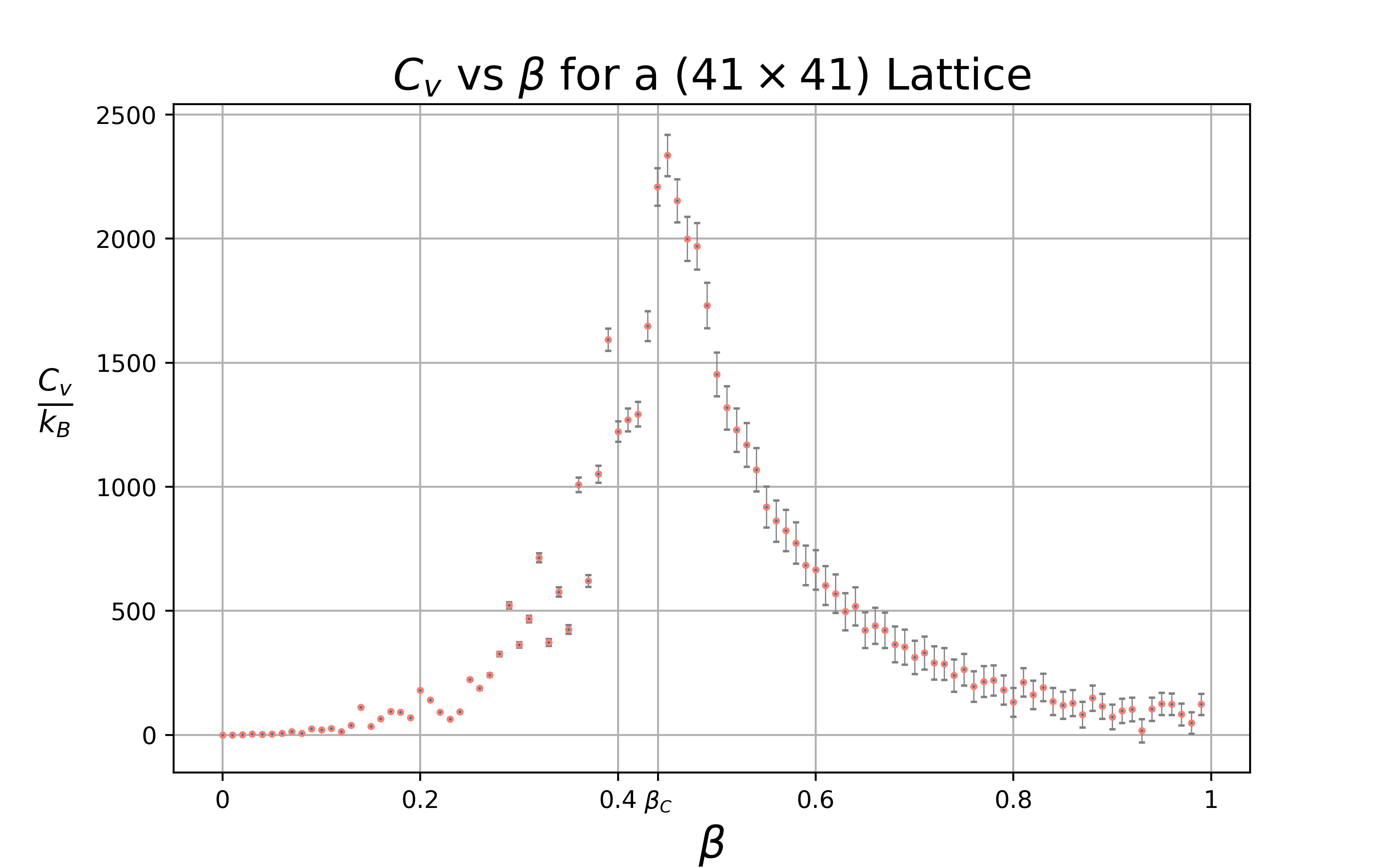
The specific heat appears to peak near \(\beta_C\) between \(\beta = 0.44\) and \(\beta = 0.45\). Which closely aligns with the exact solution of \(\beta_C = \frac{\ln(1 + \sqrt{2})}{2} \approx 0.44069\).

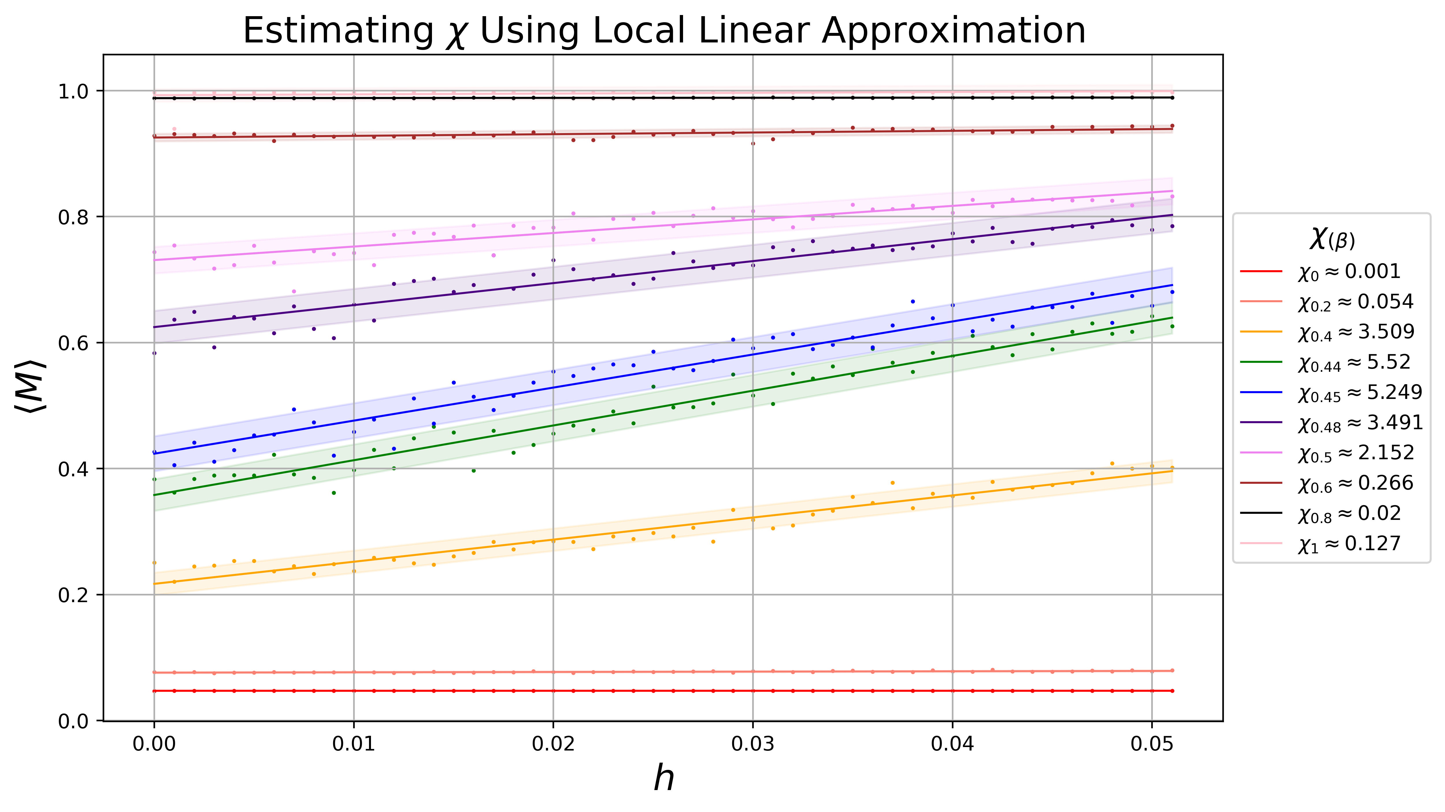
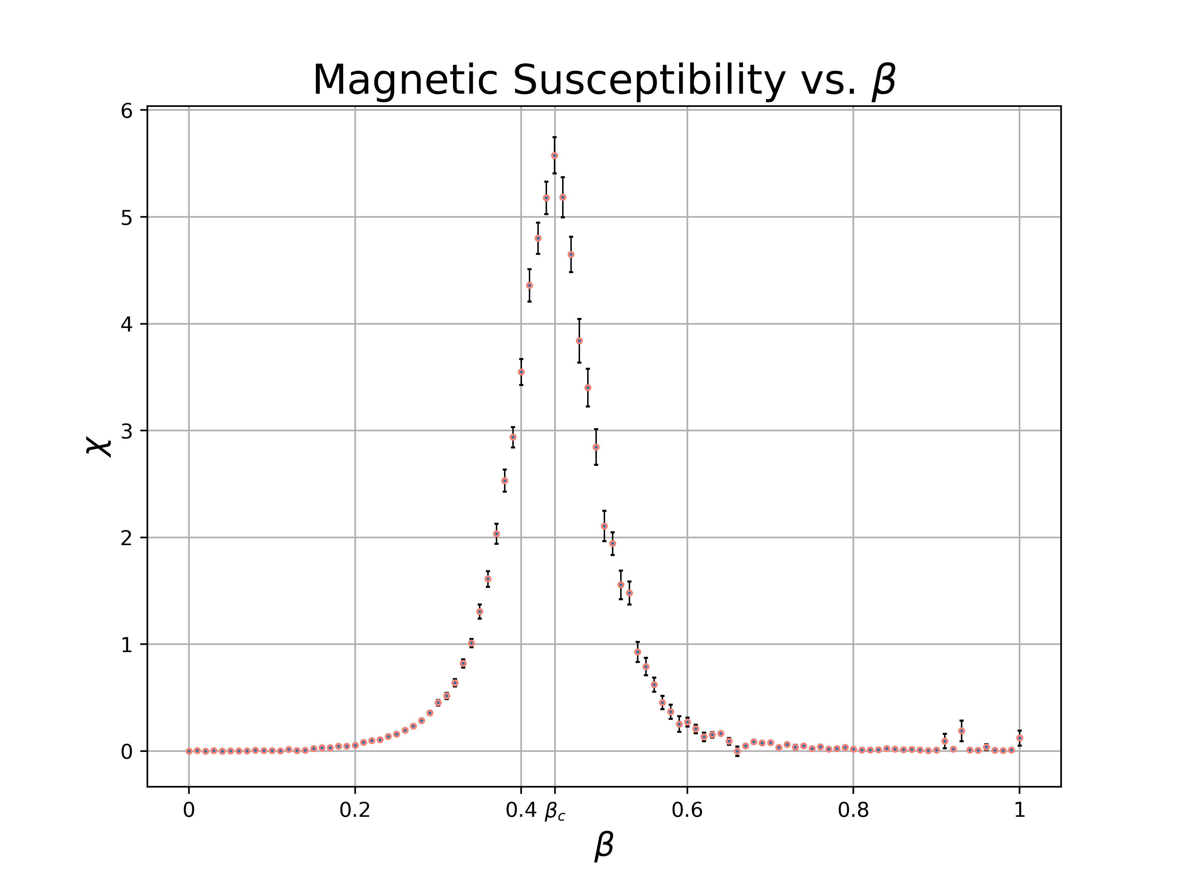
As the spins in the system can couple with an external field, \(h\), we can gain additional insight into the critical behavior of the system by manipulating the strength of the (weak) external field. Recall the full form of the Hamiltonian for our isotropic Ising model: \[ E = -J \sum_{i,j} \sigma_i \sigma_j - h \sum_{i} \sigma_i \] We can use the magnetic susceptibility, \(\chi\) to study the response of our order parameter to external perturbations. \[\chi = \frac{d \langle M \rangle}{d h} \biggm\lvert_{h=0} \] Then, for a sufficiently small interval, \(0 \lt h \lt \delta\), we can use the first order expansion: \[\langle M(h') \rangle \approx \left (\frac{d \langle M \rangle}{d h} \biggm\lvert_{h=0}\right) h' + \langle M(0) \rangle\]

I approximated the susceptibility across a range of \(\beta\) values by performing a linear fit of 50 values of \(\langle M(h) \rangle\) for \(0 \leq h \lt 0.1\). A plot containing some of the resulting fits is shown below for a few illustrative values of \(\beta\).

Renormalization Group

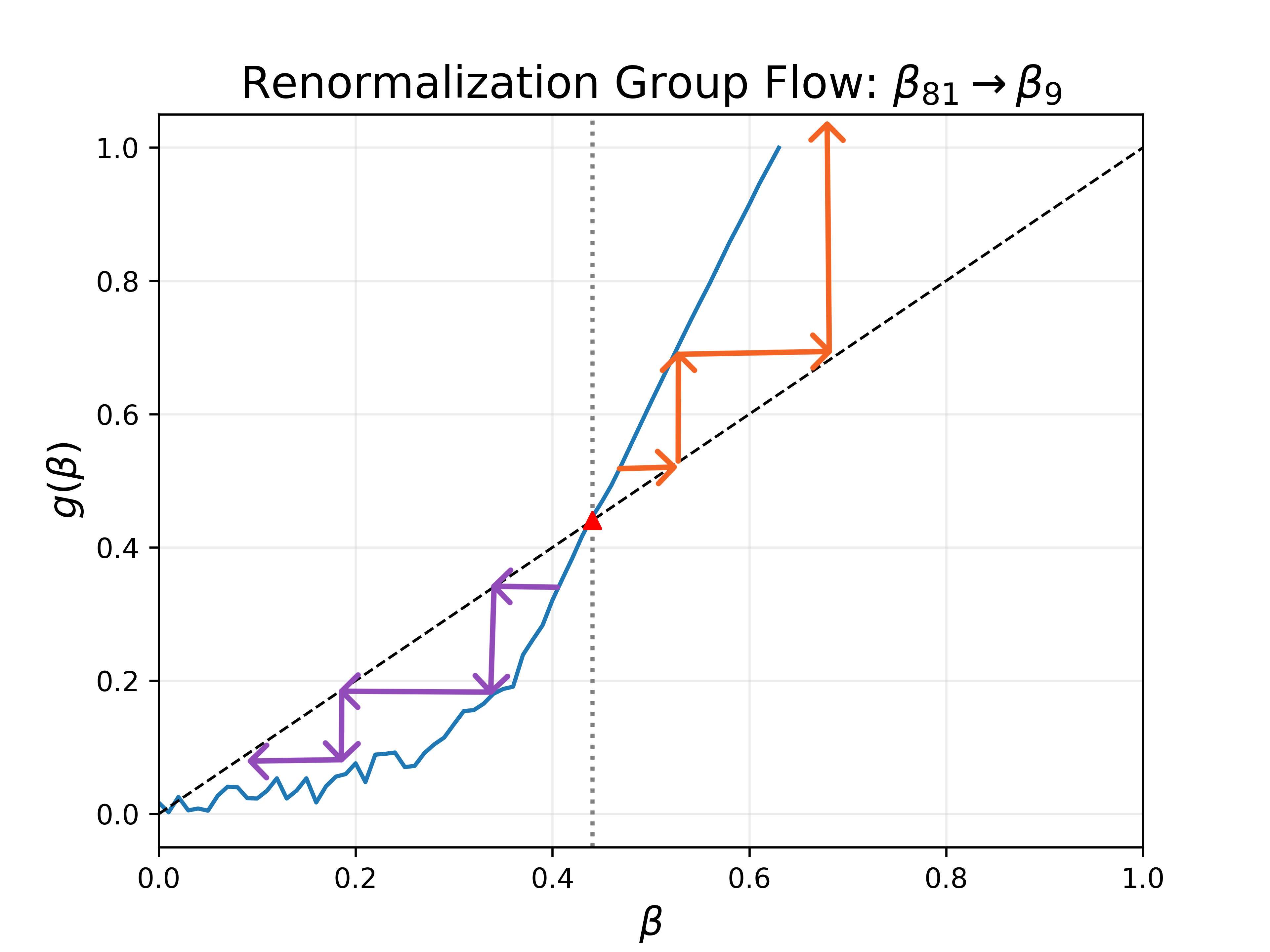
In order to get a sense of the system's properties across multiple length scales, we can use renormalization group methods such as "blocking" neighboring spins into groups, forming a smaller lattice with different properties. I grouped spins into \((9 \times 9)\) blocks with a new spin equal to the spin value shared by the majority of spins in each block. The image below (by Javier Rodríguez Laguna) illustrates the concept using a \((2 \times 2)\) grouping.

For a range of \(\beta\) values, a function \(g\) was computed by interpolating the values of \(\langle M^2(\beta) \rangle\) for the \(9 \times 9\) grid. The corresponding renormalized square magnetization values, \(\langle M_{RG}^2(\beta) \rangle\), from the larger grid were used as input for the function. The fixed points of the function, corresponding to values of beta which are mapped to itself, occur where \(g(\beta)\) intersects with \(f(\beta)=\beta\). We can see a fixed point at the critical temperature and one at \(\beta = 0\). At these temperatures, the statistics of the renormalized state look similar to an Ising system of the same dimensions. As \(g'(\beta_C) \approx 2.581 > 0\), the fixed point at the critical temperature is unstable, and repeated iterations of \(g\) look very different depending on if \(\beta \) < \(\beta_c \) or \(\beta \) > \(\beta_c \). An example flow corresponding to \(g^n(\beta)\) for \(\beta \) < \(\beta_c \) (in purple) approaches 0. On the other hand, a flow for \(\beta \) > \(\beta_c \) (in orange) diverges towards \(\infty\), approaching the uniformly magnetized state characteristic of \(T = 0\).